How to suspension nautical chart axis in Excel?
When there are boggling big or pocket-size series/points in source information, the small serial/points will non be precise enough in the chart. In these cases, some users may want to break the axis, and make both small series and large series precise simultaneously. This article will show you two means to break chart axis in Excel.
Intermission a chart axis with a secondary axis in chart
Supposing there are two data series in the source data as beneath screen shot shown, we can easily add together a chart and break the chart axis with adding a secondary axis in the chart. And you can exercise as follows:

1. Select the source data, and add a line chart with clicking the Insert Line or Area Chart (or Line)> Line on the Insert tab.

2. In the chart, right click the beneath series, and then select the Format Information Series from the right-clicking card.

3. In the opening Format Data Serial pane/dialog box, cheque the Secondary Axis choice, and then close the pane or dialog box.

iv. In the chart, correct click the secondary vertical axis (the right one) and select Format Axis from the correct-clicking menu.
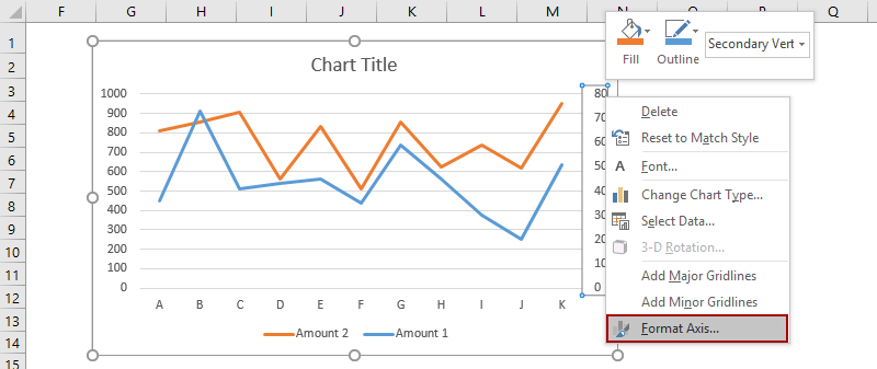
five. In the Format Centrality pane, type 160 into the Maximum box in the Premises section, and in the Number grouping enter [<=80]0;;; into the Format lawmaking box and click the Add button, and and then shut the pane.

Tip: In Excel 2010 or before versions, it will open up Format Axis dialog box. Please click Axis Option in left bar, check Fixed selection backside Maximum and so type 200 into following box; click Number in left bar, type [<=80]0;;; into the Format code box and click the Add button, at last close the dialog box.
6. Right click the principal vertical axis (the left one) in the chart and select the Format Axis to open the Format Axis pane, then enter [>=500]0;;; into the Format Code box and click the Add push button, and close the pane.
Tip: If y'all are using Excel 2007 or 2010, right click the primary vertical axis in the chart and select the Format Axis to open up the Format Axis dialog box, click Number in left bar, type [>=500]0;;; into the Format Lawmaking box and click the Add push, and close the dialog box.)
And then you lot volition see at that place are ii Y axes in the selected nautical chart which looks like the Y axis is broken. See below screen shot:

Relieve created break Y axis nautical chart as AutoText entry for easy reusing with only ane click
In addition to saving the created suspension Y centrality chart as a chart template for reusing in hereafter, Kutools for Excel's AutoText utility supports Excel users to save created chart as an AutoText entry and reuse the AutoText of chart at any time in whatever workbook with but one click. Free Trial thirty Days Now! Purchase Now!

Kutools for Excel - Includes more than 300 handy tools for Excel. Full characteristic free trial 30-mean solar day, no credit card required! Get It Now
Break axis with adding a dummy axis in nautical chart
Supposing at that place is an extraordinary large data in the source data as below screen shot, we can add a dummy axis with a suspension to make your chart centrality precise enough.
1. To break the Y axis, nosotros have to determine the min value, break value, restart value, and max value in the new broken axis. In our example we get 4 values in the Range A11:B14.

ii. Nosotros need to refigure out the source information as below screenshot shown:
(one) In Cell C2 enter =IF(B2>$B$13,$B$13,B2), and drag the Fill up Handle to the Range C2:C7;
(2) In Cell D2 enter =IF(B2>$B$13,100,NA()), and drag the Fill Handle to the Range D2:D7;
(3) In Cell E2 enter =IF(B2>$B$xiii,B2-$B$12-1,NA()), and drag the Make full Handle to the Range E2:E7.

3. Create a chart with new source information. Select Range A1:A7, so select Range C1:E7 with property the Ctrl key, and insert a chart with clicking the Insert Column or Bar Chart (or Column)> Stacked Column.

4. In the new chart, right click the Break serial (the ruby one) and select Format Data Serial from the right-clicking carte du jour.
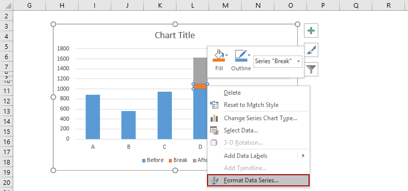
5. In the opening Format Data Series pane, click the Colour button on the Fill & Line tab, and then select the same color every bit background colour (White in our example).
Tip: I you are using Excel 2007 or 2010, it will open the Format Data Series dialog box. Click Make full in left bar, and so cheque No fill option, at last close the dialog box.)
And change the After series' color to the aforementioned color as Before serial with aforementioned way. In our example, we select Blue.

half dozen. Now we need to figure out a source information for the dummy axis. We list the data in the Range I1:K13 as below screen shot shown:
(1) In the Labels column, Listing all labels based on the min value, intermission value, restart value, and max value nosotros listed in Stride 1.
(2) In the Xpos column, blazon 0 to all cells except the broken cell. In broken cell type 0.25. Encounter left screen shot.
(3) In the Ypos column, type numbers based on the labels of Y axis in the stacked chart.

7. Right click the chart and select Select Data from right-clicking menu.

8. In the popping upwards Select Information Source dialog box, click the Add button. At present in the opening Edit Series dialog box, select Cell I1 (For Broken Y Axis) as series name, and select Range K3:K13 (Ypos Column) as series values, and click OK > OK to shut two dialog boxes.


9. Now get back to the chart, right click the new added serial, and select Alter Series Chart Type from correct-clicking carte du jour.
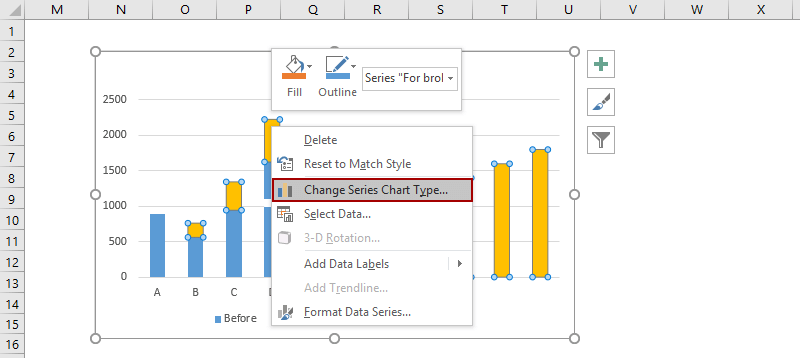
10. In the opening Change Chart Type dialog box, go to the Choose the chart blazon and centrality for your information series department, click the For Broken Y axis box, and select the Scatter with Straight Line from the drop downward list, and click the OK button.

Note: If you are using Excel 2007 and 2010, in the Change Nautical chart Type dialog box, click X Y (Scatter) in left bar, then click to select the Besprinkle with Straight Line from the drib downwards list, and click the OK push button.
11. Right click the new series once again, and select the Select Information from correct-clicking carte du jour.

12. In the Select Information Source dialog box, click to select the For broken Y centrality in the Legend Entries (Serial) department, and click the Edit button. Then in the opening Edit Serial dialog box, select Range J3:J13 (Xpos column) every bit Series X values, and click OK > OK to shut two dialog boxes.

13. Correct click the new scatter with straight line and select Format Information Series in correct-clicking carte.

14. In the opening Format Data Series pane in Excel 2013, click the colour push on the Fill & Line tab, and so select the same color as the Before columns. In our example, select Bluish. (Annotation: If you are using Excel 2007 or 2010, in the Format Data Series dialog box, click Line color in left bar, check Solid line choice, click the Colour button and select the same color equally before columns, and close the dialog box.)

fifteen. Keep selecting the scatter with straight line, and then click the Add Chart Element > Data Labels > Left on the Design tab.
Tip: Click Data Labels > Left on Layout tab in Excel 2007 and 2010.

xvi. Alter all labels based on the Labels cavalcade. For instance, select the characterization at the peak in the chart, and then type = in the format bar, then select the Cell I13, and printing the Enter key.
16. Delete some chart elements. For example, select original vertical Y axis, so press the Delete primal.

At final, you volition see your chart with a broken Y axis is created.
Relieve created break Y axis chart every bit AutoText entry for like shooting fish in a barrel reusing with merely 1 click
In addition to saving the created break Y axis chart as a chart template for reusing in future, Kutools for Excel's AutoText utility supports Excel users to save created nautical chart as an AutoText entry and reuse the AutoText of chart at any time in any workbook with only one click. Free Trial 30 Days At present! Buy Now!

Kutools for Excel - Includes more than 300 handy tools for Excel. Total feature gratuitous trial 30-day, no credit card required! Get It At present
Demo: Break the Y axis in an Excel chart
Demo: Break the Y axis with a secondary centrality in chart
Kutools for Excel includes more than 300 handy tools for Excel, free to attempt without limitation in 30 days. Download and Free Trial Now!
Demo: Break the Y centrality with adding a dummy axis in chart
Kutools for Excel includes more than 300 handy tools for Excel, gratis to endeavour without limitation in 30 days. Download and Free Trial Now!
Related Articles
The Best Part Productivity Tools
Kutools for Excel Solves Most of Your Bug, and Increases Your Productivity past lxxx%
- Reuse: Quickly insert complex formulas, charts and anything that you have used before; Encrypt Cells with password; Create Mailing List and send emails...
- Super Formula Bar (easily edit multiple lines of text and formula); Reading Layout (easily read and edit large numbers of cells); Paste to Filtered Range...
- Merge Cells/Rows/Columns without losing Information; Split Cells Content; Combine Duplicate Rows/Columns... Forbid Duplicate Cells; Compare Ranges...
- Select Duplicate or Unique Rows; Select Blank Rows (all cells are empty); Super Find and Fuzzy Find in Many Workbooks; Random Select...
- Exact Copy Multiple Cells without changing formula reference; Automobile Create References to Multiple Sheets; Insert Bullets, Check Boxes and more...
- Extract Text, Add Text, Remove by Position, Remove Space; Create and Print Paging Subtotals; Catechumen Between Cells Content and Comments...
- Super Filter (relieve and apply filter schemes to other sheets); Advanced Sort past month/calendar week/mean solar day, frequency and more; Special Filter past bold, italic...
- Combine Workbooks and WorkSheets; Merge Tables based on key columns; Separate Data into Multiple Sheets; Batch Catechumen xls, xlsx and PDF...
- More than 300 powerful features. Supports Office/Excel 2007-2019 and 365. Supports all languages. Easy deploying in your enterprise or organization. Full features 30-24-hour interval gratis trial. sixty-mean solar day money back guarantee.
")
Function Tab Brings Tabbed interface to Office, and Make Your Piece of work Much Easier
- Enable tabbed editing and reading in Word, Excel, PowerPoint , Publisher, Admission, Visio and Project.
- Open and create multiple documents in new tabs of the aforementioned window, rather than in new windows.
- Increases your productivity by 50%, and reduces hundreds of mouse clicks for you every day!
")

